Friday, 17 January 2025

First-Order IVP ODE Solution using Runge-Kutta RK4 Method

Topic: Numerical Solution to Ordinary Differential Equation

Subject: Numerical Methods

Tool: Scilab

By: Gani Comia, Jan. 2025

The 4th -order Runge-Kutta methods (RK4) is a popular and most widely used numerical technique of approximating solution to the initial value problem (IVP) of 1st -order ordinary differential equation (ODE). This article presents the equations and algorithm to apply the RK4 to a problem using Scilab scripts.

The RK4 method estimates the solution \(y=f(x)\) of an ODE with initial value condition (IVC) of the form:

$$\frac{dy}{dx}\,=\,f(x,y), \quad y(x_0)\,=\,y_0  \tag{1}$$

The RK4 algorithm requires a set of approximate values \((k_1, \; k_2, \; k_3, \; \text{and} \; k_4)\) of the slope of the solution curve at different points within the current step over an interval, \(h\).

$$\begin{aligned}k_1 &= h \cdot f \left( x_n, y_n \right) \\ k_2 &= h \cdot f \left( x_n + \frac{h}{2}, y_n+\frac{k_1}{2} \right)  \\ k_3 &= h \cdot f \left( x_n + \frac{h}{2}, y_n + \frac{k_2}{2} \right) \\ k_4 &= h \cdot f \left( x_n + h , y_n + k_3 \right) \end{aligned} \tag{2}$$

The \(k\) values from Equation (2) are then weighted and combined using Equation (3) to determine the estimates for \(y_{n + 1}\) of the numerical solution and \(x_{n + 1}\) is updated as per Equation (4).

$$y_{n+1} = y_n + \frac{1}{6} \left( k_1 + 2 k_2 + 2 k_3 + k_4 \right)  \tag{3}$$

$$x_{n+1} = x_n + h  \tag{4}$$

Let us apply using Scilab scripting the implementation of approximating solution to the ODE with initial condition in Equation (5) using the RK4 solution algorithm.

$$\frac{dy}{dx} = \frac{2x}{y} - xy , \quad y(0) = 1  \tag{5}$$

  • Scilab Script

The first block of the script is the function definition in Scilab of Equation (5).

clear;clc;

// (1) 1st-order ODE (dy/dx = f(x, y)) in Scilab form
function dydx=f(x, y)
    dydx = (2*x./y)-(x.*y);     // Example: dy/dx = 2x/y - xy
endfunction

The RK4 solution algorithm is defined in Scilab and shown in the second block of script.

// (2) Scilab function of Runge-Kutta 4th order method (RK4)
function [x, y]=rk4(f, x0, y0, h, n)
    x = zeros(1, n+1);
    y = zeros(1, n+1);
    x(1) = x0;
    y(1) = y0;

    for i = 1:n
        k1 = h * f(x(i), y(i));
        k2 = h * f(x(i) + h/2, y(i) + k1/2);
        k3 = h * f(x(i) + h/2, y(i) + k2/2);
        k4 = h * f(x(i) + h, y(i) + k3);

        x(i+1) = x(i) + h;
        y(i+1) = y(i) + (k1 + 2*k2 + 2*k3 + k4) / 6;
    end
endfunction

Initial conditions and RK4 parameters such as step size and number of intervals are shown below.

// (3) initial conditions and parameters
x0 = 0;                         // initial value of x
y0 = 1;                         // initial value of y
h = 0.1;                        // step size
n = 50;                         // no. of interval

Scilab function for the RK4 algorithm is executed to find the solution vectors for both \(x\) and \(y\) variables. Displaying on the Scilab console the last element of the variables provides an insight for the domain and range of the graph.

// (4) numerical solution to the 1st-order ODE IVP using RK4
[x, y] = rk4(f, x0, y0, h, n); 
disp(x($),y($));        // console display of the last value of x & y

Finally, visualization of numerical solutions requires plotting values of variables using appropriate graph. Shown in Figure 1 is the solution to the given ODE with IVC at \((0,1)\).

// (5) plot of the solution
clf;
f = gcf();
f.figure_size = [600,600];

plot(x, y,"b-","linewidth",3);
xlabel("$\large\textbf{x-value}$");
ylabel("$\large\textbf{y-value}$");
title("$\large\text{Solution to}\;\frac{dy}{dx}=\frac{2x}{y}-{xy}$");
legend("$\LARGE{y\,=\,f(x)}\;\text{with RK4}$",with_box=%F);
xstring(2.75,1.05,"https://gani-mech-toolbox.blogspot.com");
xgrid(3,1);

ax = gca();
ax.data_bounds = [0 1; 5 1.5];

  • Scilab Output (Figure 1)

Figure 1. Solution Plot of 1st-order ODE with IVC using RK4.

RK4 solution to 2nd-order ODE with IVC shall be presented in our next article.

Feel free to comment for inquiry, clarification, or suggestion for improvement. Drop your email to request the soft copy of the file.

Saturday, 11 January 2025

Vacuum Pump Sizing – Pumping Speed and Evacuation Time

Topic: Evacuation Time for Vacuum Pressure and Pumping Speed

Subject: Thermodynamics

Tool: Scilab

By: Gani Comia, Jan. 2025

Vacuum process creates a volume of lower pressure than the atmospheric conditions surrounding it. Atmospheric pressure, also known as air pressure, is the pressure within the Earth’s atmosphere. The standard atmosphere, which is equivalent to 1 atm or 760 Torr, is roughly equivalent to Earth’s atmospheric pressure at sea level. This article will use mTorr (millitorr) as a unit of measurement for vacuum pressure. A pressure below 760,000 mTorr (or 1 atm) is considered in vacuum state.

In an ideal condition wherein gas loads (leakage and outgassing) and pipe conductance can be considered negligible, the relationship between vacuum pressures and evacuation time can be represented by an ordinary differential equation (ODE) as shown in Equation (1).

$$\frac{dP}{dt}\;=\;-\frac{C}{V}\,P  \tag{1}$$

Where:

\(P\) - vacuum pressure at time, \(t\)
\(C\) - pumping speed of vacuum pump
\(V\) - volume of chamber to be evacuated

The analytical solution to the ODE shown in Equation (2) will be used for sizing a vacuum pump. Vacuum pumps are primarily rated based on its peak pumping speed in volume per unit of time (e.g. \(m^3/hr\), \(l/min\), \(cfm\), etc.).  Selection of the required pumping speed depends on the required evacuation time. The ultimate vacuum pressure needed will determine other vacuum system’s set-up and parameters recommended by the pump makers.

$$\large P(t)\;=\;P_0\;e^{-\left(\frac{C\,t}{V}\right)}  \tag{2}$$

Where:

\(P_0\) - initial pressure

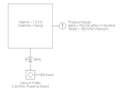
Figure 1 is a sample scenario where in different vacuum pump models will be evaluated to estimate the evacuation time for the given chamber volume size and vacuum pressure.

Figure 1. Illustrated Problem for Vacuum Pump Sizing.

The Scilab plotting capability facilitates visualizing and comparing different vacuum pump speed or capacity for the required vacuum pressure and evacuation time. Figure 2 shows the comparison of the three models, named as model X, Y, and Z, in achieving the required vacuum pressure. The evacuation time will determine the necessary peak pumping speed and thereby its model from the pump makers.

Below is the Scilab script and calculation to recreate Figure 2. The script with minor changes can be used for a different scenario defined by a design engineer.

Figure 2. Evacuation Time for 100 mTorr and Vacuum Pump Speed.

Scilab Script:

The first block of the script defines the vacuum pump speed and the physical parameter under consideration.

clear;clc;

// (1) vacuum pump specs & physical parameters
X = 3.7*1.7;            // m3/hr (from cfm), model X pumping speed
Y = 5.9*1.7;            // m3/hr (from cfm), model Y pumping speed
Z = 8.4*1.7;            // m3/hr (from cfm), model Z pumping speed

C = [X Y Z];            // m3/hr, vacuum speed capacity in row vectors   
nC = length(C);         // no. of elements of variable C
V = 1.2;                // m3, volume to be evacuated
p0 = 760000;            // mTorr, initial pressure (1 std atm)
t_end = 4;              // hr, max evacuation time, plot consideration
dt = 0.1;               // hr, time step
t = 0:dt:t_end;         // hr, time vector

Calculation of vacuum pressure for a given time domain using Equation (2) are written on the script below.

// (2) use of analytical solution to ODE and plotting
clf;
f = gcf()
f.figure_size = [600,600]

for i = 1:nC
    p(i,:) = p0 * exp(-C(i).*t./V);     // pressure @ specific time
    plot(t, p(i,:), "b-o", "linewidth",1.75);
end

xlabel("Time [ hour ]","fontsize",3);
ylabel("Vacuum Pressure [ mTorr ]","fontsize",3);
title("Evacuation Time for Vacuum Pump Model X, Y & Z");
xgrid(3,1)

Calculation of evacuation time for the required vacuum pressure are interpolated using Scilab \(interp1()\) function. Results of calculations are plotted on the graph.

// (3) interpolation of evac time @ p = 100 mTorr
format(4)
px = 100;               // mTorr, target vacuum pressure
for j = 1:nC
    tx(j,:) = interp1(p(j,:), t, px);      
    disp(tx(j,:), px)
    plot(tx(j,:),px,"marker","s","markerFaceColor","red")
    note = ["t =",string(tx(j,:)),"hr @ C =",string(C(j)),"m3/hr"]
    xstring(tx(j,:)+0.1,px,note,-50) 
end

The following block of script are for additional labels of information and plot size in terms of minimum and maximum value of pressure and time on the graph.

// (4) additional labels or informations on graph
note1 = ["$\Large\frac{dP(t)}{dt}=-\frac{C}{V}\;P(t)$"];
legend(note1,with_box = %F)
note2 = "https://gani-mech-toolbox.blogspot.com";
xstring(2.25,235,note2);
note3 = ["VP#X, C=6.3 M3H";"VP#Y, C=10 M3H";"VP#Z, C=14 M3H"];
xstring(3,50,note3);

ax = gca()
ax.data_bounds = [t(1) 0; t($) p0/3000];
This Scilab script is a useful tool for visualizing solution data and calculating specific condition.

Feel free to comment for inquiry, clarification, or suggestion for improvement. Drop your email to request the soft copy of the file.


Saturday, 4 January 2025

Free-Falling Body under Gravitational Field

Topic: Gravitational Interaction

Subject: Physics

Tool: Scilab

by:  Gani Comia, Jan. 2025

A free-falling body or object falls to the ground under the sole influence of gravity. Air resistance or any form of propulsion that acted on the object are not considered in this concept. The ordinary differential equation (ODE) in equation (1) helps explain the motion of objects in a gravitational field. The acceleration due to gravity, denoted by “\(g\)”, is approximately equal to \(\text{9.8}\;m/s^2\) on the surface of the Earth.

$$\frac{d^2 y}{dt^2}\;=\;-\;g \tag{1}$$

Solution to the given 2nd-order ODE will be based on the initial conditions as shown in equation (2).

$$\left(\;t_0 = t,\;y_0 = y,\;\frac{dy}{dt}(t_0) = v \right) \tag{2}$$

The 2nd-order ODE needs to be transformed in the system of 1st-order ODE before using it to the Scilab’s \(ode()\) function. Figure 1 which shows the position and velocity over time domain is the solution to the ODE. Instantaneous position and velocity at t = 60 sec are plotted on the graph as an example.

Figure 1. Solution to 2nd – order ODE representing Free-Falling Body.

Scilab's Script:

The first block on the script is the re-written 2nd-order ODE in the system of 1st-order ODE’s.

clear;clc;
// y'' = -g                 2nd-order ODE model for free-falling body
// y(0) = 0                 initial position
// y'(0) = 0                initial velocity

// (1) system of 1st-order ODEs equivalent to 2nd-order ODE
function dydt=freeFall(t, y)
    g = 9.8;                // m/s^2, gravitational acceleration
    dydt(1) = y(2);         // dy/dt = v
    dydt(2) = -g;           // dv/dt = -g
endfunction

Time domain considered for this solution is from 0 to 120 seconds and the initial conditions are shown in equation (3).

$$\left(\;t_0 = 0,\;y_0 = 0,\;\frac{dy}{dt}(0) = 0 \right) \tag{3}$$

Its Scilab script is shown below.

// (2) time domain and initial conditions
t = 0:0.1:120;              // sec, time span
t0 = 0;                     // sec, initial time
y0 = [0; 0];                // initial position and velocity

Scilab’s \(ode()\) function is written on below script for the solution.

// (3) solution to ode
y = ode(y0, t0, t, freeFall)

The succeeding scripts are for Scilab plotting and calculation of the instantaneous position and velocity using interpolation. Solution vectors representing position and velocity are given in the variables \(y(1,:)\) and \(y(2,:)\) respectively. The function \(interp1()\) is used for interpolation at t = 60 sec.

// (4) plot size
clf;
f=gcf();
f.figure_size=[600,700];

// (5) time and displacement plot
subplot(2,1,1)
plot(t,y(1,:),"b-","linewidth",3)
title("$\large\text{Displacement, Free-Falling Body}$")
ylabel("Displacement [m]","fontsize",3)
legend(["$\LARGE {y}$"],with_box = %F)
xgrid(3,1)

// (6) time and velocity plot
subplot(2,1,2)
plot(t,y(2,:),"r-","linewidth",3)
title("$\large\text{Velocity, Free-Falling Body}$")
xlabel("Time [sec]","fontsize",3)
ylabel("Velocity [m/sec]","fontsize",3)
legend(["$\LARGE\frac{dy}{dt}$"],with_box = %F)
xgrid(3,1)
xstring(70,-400,["https://gani-mech-toolbox.blogspot.com"])

// (7) interpolating position, Yx, and its velocity, Vx
format(8)
tx = 60;                            // sec, sample time
Yx = interp1(t, y(1,:), tx);        // m, distance
Vx = interp1(t, y(2,:), tx);        // m/s^2, velocity
disp(tx, Yx, Vx)

// (8) plot of interpolated data, time and position
subplot(2,1,1)
vertLnXs = [tx tx]; vertLnYs = [0 Yx];
horLnXs = [0 tx]; horLnYs = [Yx Yx];
plot(vertLnXs, vertLnYs,"m--","linewidth",1.25)
plot(horLnXs, horLnYs,"m--","linewidth",1.25)
plot(tx,Yx,"mo")
xstring(tx+1,Yx,["y = "+string(Yx)+" m @ 60 sec"])
a = gca();
a.children.children.mark_background = 1;

// (9) plot of interpolated data, time and velocity
subplot(2,1,2)
vertLnXs = [tx tx]; vertLnYs = [0 Vx];
horLnXs = [0 tx]; horLnYs = [Vx Vx];
plot(vertLnXs, vertLnYs,"m--","linewidth",1.25)
plot(horLnXs, horLnYs,"m--","linewidth",1.25)
plot(tx,Vx,"mo")
xstring(tx+1,Vx,["dy/dt = "+string(Vx)+" m/sec @ 60 sec"])
a = gca();
a.children.children.mark_background = 1;
For the next article, introduction of air resistance to the ODE representing the free-falling body will be presented.

Feel free to comment for inquiry, clarification, or suggestion for improvement. Drop your email to request the soft copy of the file.

A Shooting Method Approach to Boundary-Value ODEs

Topic: Differential Equations Boundary-Value Problems Subject: Numerical Methods Tool: Scilab By: Gani Comia, July 2025 The Shooting Me...