Showing posts with label Heat Transfer. Show all posts

Tuesday, 31 December 2024

Laplace Equation 1D for Steady-State Heat Conduction Model in BVP PDE

Topic: Steady-State Heat Conduction

Subject: Heat Transfer and Numerical Methods

Tool: Scilab

By: Gani Comia, Jan. 2025

The steady-state heat conduction model, as represented by the Laplace equation in one dimension (1D), is the simplest partial differential equation (PDE) you may encounter solving. This equation explains the temperature characteristics or profile between the boundaries of the given domain. Presented in this article is the application of the Laplace equation in 1D using the Finite Difference Method (FDM) for the solution.

The Laplace equation in 1D for the steady-state heat conduction is shown in Equation (1).

$$\frac{\partial^2 u}{\partial x^2}\;=\;0 \tag{1}$$

The second-order PDE in 1D can also be written in ordinary differential equations (ODE). This can be approximated using the FDM shown in Equation (2).

$$\frac{d^2 u}{d x^2}\; \approx \; \frac{u_{i+1} - 2 u_i + u_{i-1}}{\left(\Delta x\right)^2}\;=\;0 \tag{2}$$

This leads to the solution in Equation (3),

$$u_i\;=\; \frac{u_{i+1} + u_{i-1}}{2} \quad for \quad i\;=\;2,3, \ldots ,N-1 \tag{3}$$

With boundary conditions,

$$u_1\;=\;u_1, \quad u_N\;=\;u_L \tag{4}$$

Let us illustrate an example of steady-state heat conduction as shown in Figure (1) and apply the FDM solution to understand its temperature profile between boundaries. The Scilab script to implement the solution will be explained in detail in relation to the Laplace equation in 1D.

Figure 1. Sample Domain under Steady-State Heat Conduction

The solution using the Scilab script is shown below. A short explanation is provided for each code snippet.

Scilab Script.

clear;clc;clf;

// (1) primary & derived parameters
L = 100;                            // mm, length of workpiece
Nx = 11;                            // unit, number of nodes
dx = L / (Nx - 1);                  // mm, spatial step

Equation (5) is the boundary condition for this problem.

$$u_1\;=\;u_1, \quad u_{2,3, \dots ,N-1,N}\;=\;u_L \tag{5}$$

// (2) boundary temperature conditions
u = zeros(Nx, 1) + 25;              // node temp cond @ 25 deg C
u(1) = 100;                         // boundary temperature

The temperature condition at node points between boundaries can be solved using the "for-end” function of the Scilab.

// (3) temperature profile at node points using FDM
for i = 2:Nx-1
    u(i) = (u(i+1) + u(i-1))/2;
end

Below is the script for plotting the temperature profile.

// (4) plotting of temperature at node points
f = gcf()
f.figure_size = [600,600]

len = linspace(0,L,Nx);
plot(len, u, 'r-o');
title("Temperature Profile @ Eleven (11) Node Points","fontsize",3)
xlabel("Length, x [ mm ]","fontsize",3)
ylabel("Temperature, T [ C ]","fontsize",3)
xstring(58,73,"https://gani-mech-toolbox.blogspot.com")
eqn = ["$\LARGE \;\frac{\partial^2\,T}{\partial x^2}\,=\,0$"]
legend(eqn,with_box=%f)
xgrid(3,1)

a = gca()
a.data_bounds = [0 0; L max(u)]
a.children.children.mark_background = 9;

Figure (2) is the resulting plot from executing the whole script.


Figure 2. Graphical Solution for Laplace 1D using FDM with 11 Node Points

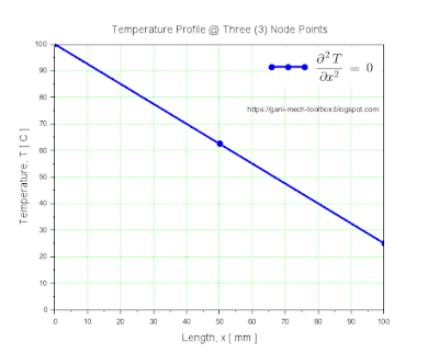
The given boundary conditions in Equation (5) will result in a curved-like temperature profile. If Equation (4) is considered as boundary conditions with the corresponding change in primary and derived parameters, specifically reducing the number of node points to 3, a linear temperature profile will become the solution.

Below is the modified script for 3 node points.

// (1) primary & derived parameters
L = 100;                            // mm, length of workpiece
Nx = 3;                             // unit, number of nodes
dx = L / (Nx - 1);                  // mm, spatial step

Figures (3) and (4) are the illustration and graphical solution for 3 node points leading to a linear temperature profile.

Figure 3. Sample Domain with 3 Node Points under Steady-State Heat Conduction


Figure 4. Graphical Solution to Laplace 1D using FDM for 3 Node Points

The number of node points taken into consideration in solving the Laplace equation using FDM dictates the type of temperature profile, linear or curve-like. You may send a comment about the consideration for a basis as to how many node points are to be used for certain conditions of the steady-state heat conduction model.

Feel free to comment for inquiry, clarification, or suggestion for improvement. Drop your email to request the soft copy of the file.

Monday, 23 December 2024

Transient Heat Conduction using Explicit FDM Solution to Thermal Diffusion

Topic: Transient Heat Conduction & Thermal Diffusion

Subject: Heat Transfer

Tool: Scilab

By: Gani Comia, Dec. 2024

This article presents the solution to the transient heat conduction system represented by the thermal diffusion equation in one dimension shown in equation (1).

$$\frac{\partial u}{\partial t}\;=\;D\;\frac{\partial^2 u}{\partial x^2} \tag{1}$$

The diffusion equation can be solved with the explicit finite difference method (FDM) given by the equation (2).

$$u_{i}^{n+1}\;=\;u_{i}^{n}\;+\;\alpha\left(u_{i+1}^{n}\,-\,2 u_{i}^{n}\,+\,u_{i-1}^{n}\right) \tag{2}$$

In solving the explicit FDM, equation (3) which is defined as a stability factor, must be satisfied to maintain numerical stability:

$$\alpha\;\leq\frac{1}{2} \tag{3}$$

or:

$$\frac{D\,\Delta t}{\left(\Delta x\right)^2}\,\leq\,\frac{1}{2}\tag{4}$$

One may refer to the detailed discussion and derivation of numerical methods of its solution. Here we are going to present the application of solving a thermal diffusion problem in one dimension using FDM. The thermal diffusion equation governs transient heat conduction where the temperature within the material changes over time and space.

Consider an example material shown in Figure 1; the temperature at each finite or nodal point at a particular time as represented by \(T(x,t)\) can be solved by using the explicit FDM.

Figure 1. Sample Material Block with Initial and Boundary Temperature. 

Figure 2 is the solution for the illustrated problem. Shown is the temperature profile, \(T(x,t)\), for a particular period of time. For example, at t = 1 sec, the material had the initial temperature of 30 deg C, and as the time progressed, the temperature at each node point became equal to the boundary temperature. The thermal diffusion equation solves for the time the material temperature reaches the boundary condition from the initial state.

Figure 2. Graphical Plot of the Explicit FDM Solution.

Scilab is used to simulate the solution with the use of FDM. An explanation of each chunk of the program script is provided here for more clarity. First on the script are parameters that defined the physical properties of the problem.

// (1) parameters
L = 160;                        // mm, length of workpiece
Nx = 40;                        // unit, number of spatial points
Time = 1000;                    // sec, time consideration
D = 12;                         // mm^2/s thermal diffusivity of 4340

Derived parameters are secondary variables calculated for explicit FDM.

// (2) derived parameters
dx = L / (Nx - 1);              // mm, spatial step
alpha = 0.5;                    // stability factor
dt = alpha .* dx.^2 ./ D;       // sec, time step for stability factor

Initial and boundary temperature conditions are provided as row vectors of the size of spatial points.

// (3) initial and boundary conditions
u = zeros(Nx, 1) + 30;          // initial temperature @ 30 deg C
u(1) = 200;                     // left boundary temperature
u(Nx) = 200;                    // right boundary temperature

Temperature distributions at each time step are calculated using the for loops of the program. The plot functions are used for the visualization of the results.

// (4) temperature distribution for time steps
for n = 1:Time
    uNew = u;                   // current state of temperature
    for i = 2:Nx-1
        uNew(i) = u(i) + alpha * (u(i+1) - 2*u(i) + u(i-1));
    end
    u = uNew;                   // updated state of temperature
    
    // (5) plotting of space, time & temperature
    f = gcf()
    f.figure_size = [600,700]
    
     function plotFunc(n)
        plot(linspace(0, L, Nx), u, 'b-o');
        title("Temperature Profile @ Time = "+ string(n) + " sec")
        ylabel("Temp [ C ]")
        xgrid(1)
        a = gca()
        a.data_bounds = [0 0; L max(u)]
        a.children.children.mark_background = 9;
    endfunction
        
    select n
        case 1 then                     // @ time = 1 sec
            subplot(3,1,1)
            plotFunc(n)
        case round(Time/5) then         // @ time = 200 sec
            subplot(3,1,2)
            plotFunc(n)
        case Time then                  // @ time = 1000 sec
            subplot(3,1,3)
            plotFunc(n)
            xlabel("Length [ mm ]")
            note1 = ["https://gani-mech-toolbox.blogspot.com"]
            xstring(85,58,note1)
    end
end

Transient heat conduction is the process where the material temperature changes for a short period of time until it reaches the steady-state heat conduction, which depends on the temperature difference between boundaries.

Feel free to comment for inquiry, clarification, or suggestion for improvement. Drop your email to request the soft copy of the file.

Saturday, 14 December 2024

Temperature Data Extraction, Visualization and Analysis using Scilab

Topic: Numerical Analysis of Temperature from Data Acquisition System (DAS);

Subject: Heat Transfer;

Tool: Scilab;

By: Gani Comia, Dec. 2024;

Data acquisition devices or systems record process data over time for monitoring and analysis purposes. This article presented how the Scilab software extracts, visualizes, and analyzes temperature numerical data from a DAS.

While DAS can actually show a graph of the data in real-time, other analysis can only be done after downloading the data soft copy in .CSV format. This blog post presented the two analyses made with the use of Scilab scripting. The first analysis made was to find the specific time for a particular temperature value, and the second one was the calculation of heat rate, or the temperature change per unit time during ramp-up.

The completed plot or graph of numerical data using Scilab is shown.

Fig. 1. Scilab Plot and Analysis of Temperature Data.

Below are the code snippets or scripts for the two sample analyses made. The completed script is shown after.

Analysis (1): Finding the Time for Specific Temperature.

// ----- analysis(1) : finding time @ temp = 232 degC -----
modOvenWallTemp = round(ovenWallTemp);
id = find(modOvenWallTemp >= 232,[-1]);  // max no. of indices
timeStd(1) = time(id(1));
timeStd(2) = time(id($));

Analysis (2): Temperature per Unit Time during Ramping-up.

// ----- analysis(2) : finding heat rate in degC / min -----
tempCond = [ovenWallTemp(1) temp(2)];
timeCond = [time(1) timeStd(1)];
heatRate = diff(tempCond)./diff(timeCond);


Scilab Script (Complete):

// Copyright (C) 2024 - Gani Comia
// Date of creation: 4 Dec 2024
// Heating Oven Temperature Data Analysis using Scilab
clear;clc;
// data extraction
clear importdata;

function [data]=importdata(filename)
    data = csvRead(filename, ",", ".", "double")
endfunction

[A] = importdata("temp_profile_before_repair_xform.csv");

// assigning data to the variables
time = A(2:$,13);
ovenWallTemp = A(2:$,2);
partTemp = A(2:$,9);

// data visualization
clf;
f=gcf();
f.figure_size=[900,600];
plot(time,ovenWallTemp,"-b","linewidth",1.75)
plot(time,partTemp,"-.r","linewidth",1)
legend(["Oven Wall","Workpiece"],"in_upper_right")
title("Analysis of Oven Temperature Profile from Data Logger")
xlabel("Time [ min ]")
ylabel("Temperature [ deg C ]")
xstring(245,100,"https://gani-mech-toolbox.blogspot.com")
a=gca(); 
a.data_bounds = [0 0;400 300]; 

// additional plot properties
t = [0:60:360, 400];
temp = [0 232 300];

// temp = 232 degC horizontal lines
plot([t(1),t($)],[temp(2),temp(2)],"--g","linewidth",1)
xstring(5,232,"Std = 232 C")

// hourly verical lines
for i = 2:length(t)-1
    plot([t(i),t(i)],[temp(1),temp(3)],"--y","linewidth",1)
end

// hourly label 
minute = 60;
hour = 1;
for i = 2:length(t)-1
    note = [string(hour),"hour"];
    xstring(minute,10,note,-90);
    minute = minute + 60;
    hour = hour + 1;
end

// ----- analysis(1) : finding time @ temp = 232 degC -----
modOvenWallTemp = round(ovenWallTemp);
id = find(modOvenWallTemp >= 232,[-1]);  // max no. of indices
timeStd(1) = time(id(1));
timeStd(2) = time(id($));

// plot of analysis(1)
timeStd = [timeStd(1) timeStd(2)];
stdTemp = [232 232];
plot(timeStd, stdTemp, "ro")
xstring(timeStd(1),stdTemp(1)-15,[string(timeStd(1)),"min"])
xstring(timeStd(2),stdTemp(2),[string(timeStd(2)),"min"])
ambient = ["Ini =",string(round(ovenWallTemp(1))),"C"];
xstring(0,ovenWallTemp(1)-15,ambient)

// ----- analysis(2) : finding heat rate in degC / min -----
tempCond = [ovenWallTemp(1) temp(2)];
timeCond = [time(1) timeStd(1)];
heatRate = diff(tempCond)./diff(timeCond);

// plot of analysis(2)
plot(timeCond,tempCond,"--","color","dimgray","linewidth",2)
noteHR = ["RATE:",string(round(heatRate)),"deg C / min"]
xstring(t(2)-20,110,noteHR,-58)

A readily available program script with some minor revision can facilitate visualization and analysis of numerical data for almost similar conditions. Program or code reusability leading to short lead times of engineering analysis is one of the benefits of using a programming tools in the engineering field.

Feel free to comment for inquiry, clarification, or suggestion for improvement. Drop your email to request the soft copy of the file.


Friday, 13 December 2024

Steady-State Heat Conduction Model using FDM Solution to 2D Laplace Equation

Topic: Finite Difference Method of Laplace Equation in 2D;

Subject: Heat Transfer and Numerical Methods;

Tool: Scilab;

By: Gani Comia, Dec. 2024;

The steady-state heat conduction model can be represented mathematically by Laplace equation. Shown is the Laplace equation in 2D:

$$\frac{\partial^2 T}{\partial x^2}+\frac{\partial^2 T}{\partial y^2}\;=\;0$$

The solution, \(T(x,y)\), represents the temperature distribution. The Laplace equation can be discretized using the Finite Difference Method (FDM) to approximate the solution numerically. This article will present the Scilab script of the FDM solution to the Laplace equation.

The FDM solution for a uniform grid, \((\Delta x = \Delta y)\), with the boundary temperatures specified based on Dirichlet conditions, is shown:

$$T_{i,j}\;=\;\frac{T_{i+1,j}+T_{i-1,j}+T_{i,j+1}+T_{i,j-1}}{4}$$

The final value of  \(T(x,y)\) is the result of iteration based on the convergence criterion:

$$max\left\vert T_{i,j}^{new}\;-\;T_{i,j}^{old}\right\vert\;<\;\epsilon$$

Consider a sample 2D domain of dimensions 30x30 units with the following constant temperature conditions. 

Fig. 1. Sample 2D Domain with Constant Temperature.

Shown below is the temperature profile as represented by \(T(x,y)\) using the FDM solution to the Laplace equation.

Fig. 2. Temperature Profile \(T(x,y)\).

The Scilab script as a toolbox can be used to implement the FDM numerical solution for the steady-state heat conduction model represented mathematically using the Laplace equation.

Scilab Script

// Copyright (C) 2024 - Gani Comia
// Date of creation: 8 Dec 2024
// FDM Solution to 2D Laplace Eq, d2T/dx2 + d2T/dy2 = 0
clear;clc;
// domain and grid parameters
Lx = 30;                    // units, domain length at x-axis
Ly = 30;                    // units, domain length at y-axis
dx = 1;                     // grid spacing at x-axis
dy = 1;                     // grid spacing at y-axis
nx = Lx./dx;                // no. of grid points in x-direction
ny = Ly./dy;                // no. of grid points in y-direction
max_iter = 1000;            // max no. of iterations
tolerance = 1e-6;           // convergence tol.

// temperature field initial value
T = zeros(nx, ny);
// boundary value conditions
    T(:,1) = 0;             // T = 0 C @ y = 1
T(1,:) = 0;                 // T = 0 C @ x = 1
T(:,ny) = 0;                // T = 0 deg C @ y = 30
T(nx,:) = 100;              // T = 100 deg C @ x = 30

// finite difference method (Jacobi iteration)
for iter = 1:max_iter
    Tnew = T;
    for i = 2:nx-1
        for j = 2:ny-1
            Tnew(i,j)=0.25*(T(i+1,j)+T(i-1,j)+T(i,j+1)+T(i,j-1));
        end
    end
    // convergence check
    if norm(Tnew - T) < tolerance then
        break;
    end
    T = Tnew;
end
// calculation status 
mprintf("\n\tCalculation completed!\n")

// plot properties
clf;
f = gcf()
f.figure_size = [700,650]
ax = gca()
ax.tight_limits = ["on" "on" "off"];

// plotting results
surf(T);
title(["$Temperature\;Profile$","$T(x,y)$"],"fontsize",4);
xlabel("x-axis");
ylabel("y-axis");
zlabel("$T$");
colormap(jet);
colorbar(0,100);

Feel free to comment for inquiry, clarification, or suggestion for improvement. Drop your email to request the soft copy of the file.

Friday, 6 December 2024

Temperature Profile of Heating Device using Data Logger and Scilab

Topic: Heating Device Temperature Profiling and Analysis;

Subject: Heat Transfer;

Tool: Temperature Data Logger and Scilab;

By: Gani Comia, Dec. 2024;

Data logger nowadays has a built-in software and computer interface to visualize in real-time as in this case the temperature profile of a device being monitored. However, for data analysis and reporting, a software like Scilab comes into picture.

Presented in this article is an example of visual report of temperature data over time. Data points from the logger can be extracted in the form of .CSV file. Transforming this data may sometimes be needed before an analysis be taken. The Scilab scripting facilitates the analysis and presentation of data for reporting.

Fig.1. Temperature Profile using Scilab

Shown below is the script to generate the graph of the data points.

Scilab Script:

// Copyright (C) 2024 - Gani Comia
// Date of creation: 6 Dec 2024
// Heating Oven Temperature Profile using Data Logger & Scilab
clear;clc;
// data extraction
clear importdata;

function [data]=importdata(filename)
    data = csvRead(filename, ",", ".", "double")
endfunction

[A] = importdata("temp_profile_after_repair_xform.csv");

// data transformation
time = A(2:$,13);
ovenWallTemp = A(2:$,2);
partTemp = A(2:$,9);
// average temperature
avgWallTemp = mean(ovenWallTemp)
avgPartTemp = mean(partTemp)

// data visualization
clf;
f=gcf();
f.figure_size=[900,600];
plot(time,ovenWallTemp,"-b","linewidth",1.75)
plot(time,partTemp,"--r","linewidth",1)
legend(["Oven Wall","Workpiece"],"in_upper_right")
title("Heating Oven Temp Profile from Data Logger")
xlabel("Time [ min ]")
ylabel("Temperature [ deg C ]")

a=gca(); 
// x & y-axis range
a.data_bounds = [0 230;780 250]; 

// additional plot properties
t = 0:60:840;
temp = [230 232 250];

// hourly vertical lines
for i = 2:length(t)
    plot([t(i),t(i)],[temp(1),temp(3)],"--y","linewidth",1)
end

// target temperature horizontal lines
plot([t(1),t($)],[temp(2),temp(2)],"--k","linewidth",1)
xstring(5,232,"Std = 232 C")
xstring(625,232,"https://gani-mech-toolbox.blogspot.com")

// hourly label 
minute = 60;
hour = 1;
for i = 2:length(t)
    note = [string(hour),"hour(s)"]
    xstring(minute,235,note,-90)
    minute = minute + 60;
    hour = hour + 1;
end

// average oven temp lines
plot([t(1),t($)],[avgWallTemp,avgWallTemp],"--b","linewidth",1)
noteWall = ["Avg Wall Temp:",string(round(avgWallTemp)),"C"]
xstring(5,avgWallTemp+0.8,noteWall)

// average part temp lines
plot([t(1),t($)],[avgPartTemp,avgPartTemp],"--r","linewidth",1)
notePart = ["Avg Part Temp:",string(round(avgPartTemp)),"C"]
xstring(5,avgPartTemp+0.5,notePart)

This toolbox of Scilab script can be handy reference to analyze data points and present it in the form of graphs for better understanding of numerical data.

Feel free to comment for inquiry, clarification, or suggestion for improvement. Drop your email to request the softcopy of the file.

C++ and Python for Numerical Solution to Spring-Mass-Damper Model

Topic: SDOF Spring-Mass-Damper System Subject: Numerical Methods & Mechanical Vibration Tools: C++, CodeBlocks, GitHub Copilot, LabP...