Vacuum Pump Sizing – Pumping Speed and Evacuation Time

Topic: Evacuation Time for Vacuum Pressure and Pumping Speed

Subject: Thermodynamics

Tool: Scilab

By: Gani Comia, Jan. 2025

Vacuum process creates a volume of lower pressure than the atmospheric conditions surrounding it. Atmospheric pressure, also known as air pressure, is the pressure within the Earth’s atmosphere. The standard atmosphere, which is equivalent to 1 atm or 760 Torr, is roughly equivalent to Earth’s atmospheric pressure at sea level. This article will use mTorr (millitorr) as a unit of measurement for vacuum pressure. A pressure below 760,000 mTorr (or 1 atm) is considered in vacuum state.

In an ideal condition wherein gas loads (leakage and outgassing) and pipe conductance can be considered negligible, the relationship between vacuum pressures and evacuation time can be represented by an ordinary differential equation (ODE) as shown in Equation (1).

$$\frac{dP}{dt}\;=\;-\frac{C}{V}\,P  \tag{1}$$

Where:

\(P\) - vacuum pressure at time, \(t\)
\(C\) - pumping speed of vacuum pump
\(V\) - volume of chamber to be evacuated

The analytical solution to the ODE shown in Equation (2) will be used for sizing a vacuum pump. Vacuum pumps are primarily rated based on its peak pumping speed in volume per unit of time (e.g. \(m^3/hr\), \(l/min\), \(cfm\), etc.).  Selection of the required pumping speed depends on the required evacuation time. The ultimate vacuum pressure needed will determine other vacuum system’s set-up and parameters recommended by the pump makers.

$$\large P(t)\;=\;P_0\;e^{-\left(\frac{C\,t}{V}\right)}  \tag{2}$$

Where:

\(P_0\) - initial pressure

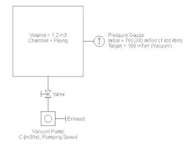
Figure 1 is a sample scenario where in different vacuum pump models will be evaluated to estimate the evacuation time for the given chamber volume size and vacuum pressure.

Figure 1. Illustrated Problem for Vacuum Pump Sizing.

The Scilab plotting capability facilitates visualizing and comparing different vacuum pump speed or capacity for the required vacuum pressure and evacuation time. Figure 2 shows the comparison of the three models, named as model X, Y, and Z, in achieving the required vacuum pressure. The evacuation time will determine the necessary peak pumping speed and thereby its model from the pump makers.

Below is the Scilab script and calculation to recreate Figure 2. The script with minor changes can be used for a different scenario defined by a design engineer.

Figure 2. Evacuation Time for 100 mTorr and Vacuum Pump Speed.

Scilab Script:

The first block of the script defines the vacuum pump speed and the physical parameter under consideration.

clear;clc;

// (1) vacuum pump specs & physical parameters
X = 3.7*1.7;            // m3/hr (from cfm), model X pumping speed
Y = 5.9*1.7;            // m3/hr (from cfm), model Y pumping speed
Z = 8.4*1.7;            // m3/hr (from cfm), model Z pumping speed

C = [X Y Z];            // m3/hr, vacuum speed capacity in row vectors   
nC = length(C);         // no. of elements of variable C
V = 1.2;                // m3, volume to be evacuated
p0 = 760000;            // mTorr, initial pressure (1 std atm)
t_end = 4;              // hr, max evacuation time, plot consideration
dt = 0.1;               // hr, time step
t = 0:dt:t_end;         // hr, time vector

Calculation of vacuum pressure for a given time domain using Equation (2) are written on the script below.

// (2) use of analytical solution to ODE and plotting
clf;
f = gcf()
f.figure_size = [600,600]

for i = 1:nC
    p(i,:) = p0 * exp(-C(i).*t./V);     // pressure @ specific time
    plot(t, p(i,:), "b-o", "linewidth",1.75);
end

xlabel("Time [ hour ]","fontsize",3);
ylabel("Vacuum Pressure [ mTorr ]","fontsize",3);
title("Evacuation Time for Vacuum Pump Model X, Y & Z");
xgrid(3,1)

Calculation of evacuation time for the required vacuum pressure are interpolated using Scilab \(interp1()\) function. Results of calculations are plotted on the graph.

// (3) interpolation of evac time @ p = 100 mTorr
format(4)
px = 100;               // mTorr, target vacuum pressure
for j = 1:nC
    tx(j,:) = interp1(p(j,:), t, px);      
    disp(tx(j,:), px)
    plot(tx(j,:),px,"marker","s","markerFaceColor","red")
    note = ["t =",string(tx(j,:)),"hr @ C =",string(C(j)),"m3/hr"]
    xstring(tx(j,:)+0.1,px,note,-50) 
end

The following block of script are for additional labels of information and plot size in terms of minimum and maximum value of pressure and time on the graph.

// (4) additional labels or informations on graph
note1 = ["$\Large\frac{dP(t)}{dt}=-\frac{C}{V}\;P(t)$"];
legend(note1,with_box = %F)
note2 = "https://gani-mech-toolbox.blogspot.com";
xstring(2.25,235,note2);
note3 = ["VP#X, C=6.3 M3H";"VP#Y, C=10 M3H";"VP#Z, C=14 M3H"];
xstring(3,50,note3);

ax = gca()
ax.data_bounds = [t(1) 0; t($) p0/3000];

This Scilab script is a useful tool for visualizing solution data and calculating specific condition.

Feel free to comment for inquiry, clarification, or suggestion for improvement. Drop your email to request the soft copy of the file.