Factor-of-Safety using Yield Stress and Maximum Shear Stress Theory

Topic: Steady Loading and Failure Theory

Subject: Machine Design

Tool: Scilab

By: Gani Comia, Feb. 2025

A static or steady load is a stationary force or moment acting on a machine or structural member. There are two approaches to calculate the margin of safety to prevent failures on the member: - factor-of-safety (\({FoS}\)) and reliability approach. These examine or compare the strength of a member and the anticipated induced stress from static loading for the selection of the optimum or suitable material and dimensions.

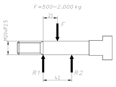
This article demonstrates the use of \({FoS}\) approach in verifying the suitability of a machine member for the given steady load. Figure 1 illustrates the condition in which the T-bolt made of AISI 1050 will be used as shackle pin to carry or lift a range of steady load from 500 to 2000 kg. The \(FoS\) approach can determine the maximum dead load the pin is capable of lifting steadily.

Figure 1. Shackle pin subjected to a steady loading.

Equations (1), (2), and (4) represent the basis for calculating \({FoS}\) from the given condition.

\({FoS}\) in Simple Tension, Compression, or Bending

$${FoS}_{bending}\;=\;\frac{\sigma_{yp}}{\sigma_{max}} \tag{1}$$

Where:
\({FoS}_{bending}\) – factor-of-safety in simple tension, compression, or bending
\(\sigma_{yp}\) – material’s yield point
\(\sigma_{max}\) – maximum induced stress

\({FoS}\) in Pure Shear

$${FoS}_{shear}\;=\;\frac{\tau_{yp}}{\tau_{max}} \tag{2}$$

Where:
\({FoS}_{shear}\) – factor-of-safety in pure shear
\(\tau_{yp}\) – material’s yield point in shear
\(\tau_{max}\) – maximum induced shear stress

\({FoS}\) using Max Shear Stress Theory

$$\tau_{mss}\;=\;\sqrt{\left(\frac{\sigma_{max}-\sigma_{min}}{2}\right)^2 + \tau_{max}^2} \tag{3}$$

$${FoS}_{mss}\;=\;\frac{\tau_{yp}}{\tau_{mss}} \tag{4}$$

Where:
\({FoS}_{mss}\) – factor-of-safety based on maximum shear stress theory
\(\tau_{mss}\) – induced stress using max shear stress theory
\(\sigma_{max}\) – stress due to bending at outermost surface of the shackle pin
\(\sigma_{min}\) – stress due to bending at neutral axis of the shackle pin

For steady loading, the recommended factor-of-safety is from 1.5 to 3.0 for the general engineering applications and ductile materials. The use of 1.5 as factor-of-safety will determine the maximum allowable steady load for a member. Presented below is the Scilab script for calculation documentation and validation of design in a typical engineering organizational setup.

Scilab Script

// Copyright (C) 2025 - Gani Comia
// Date of creation: 7 Feb 2025
// Shackle Pin Stress Analysis Rev 01
clear;clc;

// (1) Primary and secondary parameters.
d = 17.5;               // mm, minor dia for M20 thread
L = 42.0;               // mm, length under load
Wt = 500:10:2000;       // kg, weight of load
F = Wt.*9.8;            // N, load per pin
A = (%pi/4)*d.^2;       // mm^2, cross-sectional area at thread
S = (%pi/32)*d.^3;      // mm^3, section modulus of pin

// (2) Maximum moment and shear load.
Mmax = F.*L./4;         // N-mm, max moment load
V = F./2;               // N, max shear load

// (3) Bending and shear stress.
sigmaMax = Mmax./S;     // MPa, max bending stress
tauMax = (4/3)*V./A;    // MPa, max shear stress

// (4) Material properties, AISI 1050
sigmaYp = 375.0;        // MPa, yield point
tauYp = 0.5*sigmaYp;    // MPa, yield point in shear

// (5) Factor-of-safety (FoS), Bending and Pure Shear
FoSbending = sigmaYp./sigmaMax;     // factor-of-safety in bending
FoSshear = tauYp./tauMax;           // factor-of-safety in pure shear

// (6) Factor-of-safety (Fos), Max Shear Stress Theory
sigma1 = sigmaMax;          // MPa, max principal stress, outermost
sigma3 = 0;                 // MPa, min principla stress, neutral axis
tauMss = sqrt(((sigma1-sigma3)/2).^2 + tauMax.^2);  // MPa, MSST
FoSmsst = tauYp./tauMss;    // factor-of-safety in max shear stress

// (7) Plot of analysis
clf;
plot("ln",Wt,FoSmsst,"b-","linewidth",3);
plot("ln",Wt,FoSbending,"r--","linewidth",1.5);
plot("ln",Wt,FoSshear,"m-","linewidth",2.5);
note1 = ["Max Shear Stress","Bending Stress","Shear Stress"];
legend(note1,with_box=%F);
xgrid(3,0);
title("Shackle Pin FoS based on Failure Theory","fontsize",3.5);
xlabel("Lifting Load [kg]","fontsize",3);
ylabel("Factor of Safety","fontsize",3);

// Interpolating weight for the min factor-of-safety 1.5
format(6);
fos = 1.5;
wtInt = interp1(FoSmsst,Wt,fos);
disp(fos, wtInt);
xVerMin = [wtInt wtInt]; xHorMin = [400 wtInt];
yVerMin = [0 fos]; yHorMin = [fos fos]; 
plot(xVerMin, yVerMin,"b--");
plot(xHorMin, yHorMin,"b--");
plot(wtInt, fos,"marker","s","markerFaceColor","blue");
note2 = ["Max Load (kg) =",string(wtInt),"@ FoS =",string(fos)];
xstring(wtInt-50,fos+0.4,note2);
note3 = "https://gani-mech-toolbox.blogspot.com";
xstring(1200,11,note3);

Scilab Script Output (Figure 2)

Figure 2. Plot of Calculation of the Three Failure Theories.

The resulted plot shows that for a minimum factor-of-safety of 1.5, the shackle pin should only be loaded with not more than 1232 kg to prevent failure. 

Just like any engineering drawings to document the mechanical design, calculation in the form of scripts and notebooks are also kept for design review and future reference.

Feel free to comment for inquiry, clarification, or suggestion for improvement. Drop your email to request the soft copy of the file. 

Simple Harmonic Motion Solution using Runge-Kutta RK4 Method

Topic: Oscillatory Motion and Numerical Solution of ODE

Subject: Physics and Numerical Methods

Tool: Scilab

By: Gani Comia, Jan. 2025

The 4^th -order Runge-Kutta methods (RK4) is also used for numerical technique of approximating solution to the initial value problem (IVP) of 2^nd- order ordinary differential equation (ODE). This article presents the solution to the basic equation of simple harmonic motion (SHM) using RK4 algorithm in Scilab.

SHM is a form of nonhomogeneous linear differential equation (LDE) of second-order as shown in Equation (1).

$$y''\;+\;p(t)\,y'\;+\;q(t)\,y\;=\;r(t) \tag{1}$$ 

In order to solve a given higher-order differential equation, it is required to be converted to a system of first-order differential equations as presented below.

Let us define the following dependent variables, \(y_1\) and \(y_2\):

$$y_1\;=\;y \tag{2}$$

$$y_2\;=\;y' \tag{3}$$

Then, the nonhomogeneous LDE can be re-written as a system of 1^st-order ODE in Equation (4) and (5):

$$y'_1\;=\;y_2 \tag{4}$$

$$y'_2\;=\;-p(t)\,y_2\;-\;q(t)\,y_1\;+\;r(t) \tag{5}$$

With that presented, let us define and illustrate a problem using the basic equation of SHM and convert its 2^nd-order ODE to a system of 1^st-order to use the RK4 method in finding its approximate solution.

Figure 1. Single-Degree of Freedom (SDOF) Spring-Mass Model Oscillation Problem

The SDOF spring-mass model oscillation can be described by the basic equation of SHM shown in Equation (6).

$$m\,\frac{d^2y}{dt^2}\,+\,k\,y\,=\,0, \quad y(t_0)=y_0\;\;\text{and}\;\;y'(t_0)=y'_0 \tag{6}$$

Where:

\(m\) – mass

\(k\) – spring constant

\(t\) – time

\(t_0\) - initial time

\(y_0\) – initial displacement

\(y’_0\) – initial velocity

The solution to the ODE of SHM can be approximated using the Runge-Kutta (RK4) Method. The RK4 will be using the same algorithm presented in the previous article “First-Order IVP ODE Solution using Runge-Kutta RK4 Method” with the link shown: https://gani-mech-toolbox.blogspot.com/2025/01/first-order-ivp-ode-solution-using.html. Figure 2 shows the solution to the problem illustrated in Figure 1.

Figure 2. Solution to Spring-Mass Model System with RK4 using Scilab Script

The Scilab script to solve the given problem is presented below. Each block of the code is commented comprehensively for better understanding of the program sequence by the reader.

Scilab Script:

clear;clc;
// single-degree of freedom spring-mass model oscillator system
// m*y'' + k*y = 0  or  y'' + (k/m)*y = 0
// nonhomogeneous linear differential equation (LDE) of second-order
// y'' + p(t)y' + q(t)y = g(t) 
// where: p(t)=0; q(t)=k/m; g(t)=0

// (1) 2nd-order LDE re-written in the system of 1st-order ODEs
function dydt=f(t, y)
    m = 1;                  // kg, mass of the object
    k = 20;                 // N/m, spring constant
    p = 0;                  // coefficient of y'
    q = k/m;                // coefficient of y
    g = 0;                  // forcing function
    dydt = [y(2); -p*y(2) - q*y(1) + g];
endfunction

As you may compare the \(rk4\) function in block (2) to the previous article, the final time, \(t_f\), is used as one of the input arguments instead of the number of intervals, \(n\). Both \(rk4\) functions can be used to come up with the same solution.

// (2) RK4 function or algorithm for 1st-order ODEs
function [t, y]=rk4(f, t0, y0, h, tf)
    n = round((tf - t0)./h);
    t(1) = t0;          // initial time, t0
    y(:, 1) = y0;       // y(t0)=y0 & y'(t0)=y0' in column vector

    for i = 1:n
        // approximate values of slopes of solution curves
        k1 = h * f(t(i), y(:, i));
        k2 = h * f(t(i) + h / 2, y(:, i) + k1 / 2);
        k3 = h * f(t(i) + h / 2, y(:, i) + k2 / 2);
        k4 = h * f(t(i) + h, y(:, i) + k3);
        // estimates of numerical solution
        y(:, i + 1) = y(:, i) + (k1 + 2 * k2 + 2 * k3 + k4) / 6;
        t(i+1) = t(i) + h;
    end
endfunction

// (3) initial conditions and parameters
t0 = 0;             // sec, initial time
tf = 5;             // sec, final time
h = 0.01;           // sec, time step size
y0 = [0.05; 0];     // initial disp & velocity: y(0)=0.05, y'(0)=0

// (4) solution to the ODE by calling RK4 defined function
[t, y] = rk4(f, t0, y0, h, tf);

// (5) solution plot
clf;
plot(t, y(1, :),"b-","linewidth",4);       // displacement plot
plot(t, y(2, :),"r--","linewidth",1.8);    // velocity plot
xlabel("$\Large t \quad \text{(time)}$");
ylabel("$\Large y(t)\;\;\text{or}\;\;\frac{dy(t)}{dt}$");
note1 = "Spring-Mass Model System using Runge-Kutta RK4";
title(note1,"fontsize",3.5);
note2 = ["$\Large y(t)$","$\Large \frac{dy(t)}{dy}$"];
legend(note2, with_box = %F);
note3 = "https://gani-mech-toolbox.blogspot.com"
xstring(0.1,0.35,note3);
xgrid(3,1);

// (6) other plot information
disp(max(y(1,:)), min(y(1,:)))
disp(max(y(2,:)), min(y(2,:)))
ax = gca();
ax.data_bounds = [0 -0.4; 5 0.4];

// (7) natural frequency
format(5);
k = 20;                     // N/m, spring constant
m = 1;                      // kg, mass of object
omega = sqrt(k/m);          // Hz, natural frequency
disp(omega);
note4 = ["$\LARGE\mathbf{\omega_n}\;=\;\text{4.5 Hz}$"];
xstring(0.1,0.25,note4)

The Scilab script in this article can be one of your references to solve any engineering problems that can be described by the nonhomogeneous linear differential equation (LDE) of second-order.

Feel free to comment for inquiry, clarification, or suggestion for improvement. Drop your email to request the soft copy of the file.

First-Order IVP ODE Solution using Runge-Kutta RK4 Method

Topic: Numerical Solution to Ordinary Differential Equation

Subject: Numerical Methods

Tool: Scilab

By: Gani Comia, Jan. 2025

The 4^th -order Runge-Kutta methods (RK4) is a popular and most widely used numerical technique of approximating solution to the initial value problem (IVP) of 1^st -order ordinary differential equation (ODE). This article presents the equations and algorithm to apply the RK4 to a problem using Scilab scripts.

The RK4 method estimates the solution \(y=f(x)\) of an ODE with initial value condition (IVC) of the form:

$$\frac{dy}{dx}\,=\,f(x,y), \quad y(x_0)\,=\,y_0  \tag{1}$$

The RK4 algorithm requires a set of approximate values \((k_1, \; k_2, \; k_3, \; \text{and} \; k_4)\) of the slope of the solution curve at different points within the current step over an interval, \(h\).

$$\begin{aligned}k_1 &= h \cdot f \left( x_n, y_n \right) \\ k_2 &= h \cdot f \left( x_n + \frac{h}{2}, y_n+\frac{k_1}{2} \right)  \\ k_3 &= h \cdot f \left( x_n + \frac{h}{2}, y_n + \frac{k_2}{2} \right) \\ k_4 &= h \cdot f \left( x_n + h , y_n + k_3 \right) \end{aligned} \tag{2}$$

The \(k\) values from Equation (2) are then weighted and combined using Equation (3) to determine the estimates for \(y_{n + 1}\) of the numerical solution and \(x_{n + 1}\) is updated as per Equation (4).

$$y_{n+1} = y_n + \frac{1}{6} \left( k_1 + 2 k_2 + 2 k_3 + k_4 \right)  \tag{3}$$

$$x_{n+1} = x_n + h  \tag{4}$$

Let us apply using Scilab scripting the implementation of approximating solution to the ODE with initial condition in Equation (5) using the RK4 solution algorithm.

$$\frac{dy}{dx} = \frac{2x}{y} - xy , \quad y(0) = 1  \tag{5}$$

• Scilab Script

The first block of the script is the function definition in Scilab of Equation (5).

clear;clc;

// (1) 1st-order ODE (dy/dx = f(x, y)) in Scilab form
function dydx=f(x, y)
    dydx = (2*x./y)-(x.*y);     // Example: dy/dx = 2x/y - xy
endfunction

The RK4 solution algorithm is defined in Scilab and shown in the second block of script.

// (2) Scilab function of Runge-Kutta 4th order method (RK4)
function [x, y]=rk4(f, x0, y0, h, n)
    x = zeros(1, n+1);
    y = zeros(1, n+1);
    x(1) = x0;
    y(1) = y0;

    for i = 1:n
        k1 = h * f(x(i), y(i));
        k2 = h * f(x(i) + h/2, y(i) + k1/2);
        k3 = h * f(x(i) + h/2, y(i) + k2/2);
        k4 = h * f(x(i) + h, y(i) + k3);

        x(i+1) = x(i) + h;
        y(i+1) = y(i) + (k1 + 2*k2 + 2*k3 + k4) / 6;
    end
endfunction

Initial conditions and RK4 parameters such as step size and number of intervals are shown below.

// (3) initial conditions and parameters
x0 = 0;                         // initial value of x
y0 = 1;                         // initial value of y
h = 0.1;                        // step size
n = 50;                         // no. of interval

Scilab function for the RK4 algorithm is executed to find the solution vectors for both \(x\) and \(y\) variables. Displaying on the Scilab console the last element of the variables provides an insight for the domain and range of the graph.

// (4) numerical solution to the 1st-order ODE IVP using RK4
[x, y] = rk4(f, x0, y0, h, n); 
disp(x($),y($));        // console display of the last value of x & y

Finally, visualization of numerical solutions requires plotting values of variables using appropriate graph. Shown in Figure 1 is the solution to the given ODE with IVC at \((0,1)\).

// (5) plot of the solution
clf;
f = gcf();
f.figure_size = [600,600];

plot(x, y,"b-","linewidth",3);
xlabel("$\large\textbf{x-value}$");
ylabel("$\large\textbf{y-value}$");
title("$\large\text{Solution to}\;\frac{dy}{dx}=\frac{2x}{y}-{xy}$");
legend("$\LARGE{y\,=\,f(x)}\;\text{with RK4}$",with_box=%F);
xstring(2.75,1.05,"https://gani-mech-toolbox.blogspot.com");
xgrid(3,1);

ax = gca();
ax.data_bounds = [0 1; 5 1.5];

Scilab Output (Figure 1)

Figure 1. Solution Plot of 1st-order ODE with IVC using RK4.

RK4 solution to 2^nd-order ODE with IVC shall be presented in our next article.

Feel free to comment for inquiry, clarification, or suggestion for improvement. Drop your email to request the soft copy of the file.