Saturday, 30 November 2024

CNC Machining Feed Rate for Material Surface Finish in Ra using Scilab

Topic: Turning (Lathe) Feed Rate Calculation for a given Average Roughness;

Subject: Machine Shop Technology;

Tool: Scilab;

By: Gani Comia, Nov. 2024;

Average Roughness, or Ra, is a parameter to measure the surface finish of a workpiece. Ra is typically expressed in micrometers \( \mu m \). Shown here are some of the common Ra values for different surface finishes:

  • Polished; Ra 0.05~0.2 \( \mu m \)
  • Machined (Finish): Ra 0.8~3.2 \( \mu m \)
  • Machined (Rough): Ra 3.2~12.5 \( \mu m \)
  • Casted: Ra 12.5~50 \( \mu m \)
In turning metal workpieces, feed rate, f (mm/rev), is one of the considerations to achieve the required surface finish. Let us say we wanted to achieve an Ra 3.2 \( \mu m \) and we have two types of insert, round and rhombic. The machining parameter, which is feed rate, can be calculated and used in the CNC turning program. Below is the basis for calculating feed rate in mm/rev and its Scilab script.

$$f\;=\;{2}\;{\sqrt{\frac{r\;R_a}{125}}}$$


Scilab Script

// Machining Feed Rate Calculation in CNC Turning
// Gani Comia, Jan. 2023
clear;clc;

// given insert type and corner radius
// round corner, r=6.35 mm, rhombic corner, r=0.2 mm
r = [6.35 0.2];                                 // mm
// standard Ra, surface finish
Ra_std = [0.1 0.2 0.4 0.8 1.6 3.2 6.3 12.5];    // um
Ra = linspace(0.1,12.5,200);                    // um

// formula feed/rev for insert radius and Ra requirement
function f=feedPerRev(r, Ra)
    f = 2.*sqrt(r.*Ra./125);  // mm/rev, feed per rev
endfunction

// calculation of feed rate for standard Ra
f_std_round = feedPerRev(r(1), Ra_std);
f_std_rhombic = feedPerRev(r(2), Ra_std);
// table of feed rate for standard Ra
mprintf("\n Ra(um)\t\tf(mm/rev) Round\tf(mm/rev) Rhombic\n")
Table = [Ra_std' f_std_round' f_std_rhombic'];
mprintf("\n %3.2f \t\t %3.3f \t\t %3.3f\n", Table)

// calculation of feed rate from 0.1 to 12.5 um, Ra
f_round = feedPerRev(r(1), Ra);
f_rhombic = feedPerRev(r(2), Ra);

// plotting results
clf;
plot(Ra, f_round, "b-", "linewidth", 1.5)
plot(Ra, f_rhombic, "r-", "linewidth", 1.5)

title("CNC Lathe Feed Rate for Surface Finish")
xlabel(["Average Roughness", "$\Large{R_a\,\;(\mu\,m)}$"])
ylabel(["Feed Rate", "$\Large{f\,\;(mm/rev)}$"])
legend(["Round r = 6.35 mm", "Rhombic r = 0.2 mm"],2)

// case scenario for Ra=3.2 um
Ra_32 = 3.2;
f_round_32 = feedPerRev(r(1), Ra_32);
f_rhombic_32 = feedPerRev(r(2), Ra_32);

// line plot of special concern
xpt_ver = [3.2 3.2]; ypt_ver = [0 f_round_32];
plot(xpt_ver, ypt_ver, "g--")
xpt_hor = [3.2 0]; ypt_hor = [f_round_32 f_round_32];
plot(xpt_hor, ypt_hor, "g--")
xpt_hor_1 = [3.2 0]; ypt_hor_1 = [f_rhombic_32 f_rhombic_32]
plot(xpt_hor_1, ypt_hor_1, "g--")

// plotting points
plot(Ra_32, f_round_32, ".b")
xstring(0.1, f_round_32, ["$\large{f\;=\;0.806\;mm/rev}$"])
plot(Ra_32, f_rhombic_32, ".r")
xstring(0.3, f_rhombic_32, ["$\large{f\;=\;0.143\;mm/rev}$"])
xstring(3.2, 0.30, ["$\Large{R_a\;=\,3.2\;\mu\;m}$"], -90)

Visualization of the relationship of f and Ra for a given nose radius, r, in turning machining is a helpful guide for machinist reference. 

Fig. 1. Turning Feed Rate for Insert Type and Surface Finish.

This toolbox can be your handy reference to calculate the turning feed rate as the initial machining parameter in the CNC program.

Feel free to comment for inquiry, clarification, or suggestion for improvement. Drop your email to request the softcopy of the file.


Monday, 25 November 2024

Numerical Differentiation using Central Difference Method with Python

Topic: CDM of Numerical Differentiation;

Subject: Numerical Method;

Tool: Python;

by: Gani Comia, Nov. 2024;

Numerical differentiation is a method to approximate the derivative of a function using discrete data points. This is applicable for a set of data points or having a function that is difficult to differentiate analytically. There are three common methods of numerical differentiation.

  • Forward Difference
  • Backward Difference
  • Central Difference

The central difference method is generally more accurate as it considers the function values on both sides of the independent variable. The toolbox presented here is the Python script of numerical differentiation using CDM. The plot is generated for both the given function and its derivative for comparison.

Python Script

# -*- coding: utf-8 -*-
"""
Created on Tue Jun 22 19:17:34 2021
@by: Gani Comia
"""

'''
This is an example plotting script of a function and its derivative
using the central difference method (CDM) of numerical differentiation
with the use of Python.

Function:  f(x) = exp(-x^2)
Derivative:  f'(x) = (f(x+h) - f(x-h)) / 2h
'''

import numpy as np
import matplotlib.pyplot as plt

# Given: domain and the function, f(x)
x = np.linspace(-5,5,1000)            # domain from -5 to 5
f = np.exp(-x**2)                           # f(x)

# Approximation of derivative, f'(x), using numerical differentiation
h = 0.001                                      # step size
df = np.zeros(1000,float)              # initialization

# Numerical differentiation using CDM
# Note: x is replaced with x[i] and added with +h and -h
for i in np.arange(1000):
    df[i] = (np.exp(-(x[i]+h)**2) - np.exp(-(x[i]-h)**2)) / (2*h)

# Plot of f(x) and f'(x)
plt.plot(x, f, label="f(x)")
plt.plot(x, df, label="f'(x)")
plt.title("Plot of f(x) and f'(x) of $e^{(-x^2)}$")
plt.xlabel("x-value")
plt.ylabel("f(x) and f'(x)")
plt.legend()
plt.show()


Visualization of the given function and its derivative.


Fig. 1. Plot of the function and its derivative.


This kind of script can be saved and rerun to solve similar engineering problems. Python IDEs such as Thonny, Spyder, Jupyter NB, and Google Collab can be used to execute the script.

Feel free to comment for inquiry, clarification, or suggestion for improvement. Drop your email to request the softcopy of the file.


Sunday, 24 November 2024

Mechanical Vibration Measurement using Accelerometer and Scilab

Topic: Vibration Detection and Measurement;

Subject: Mechanical Vibration;

Tool: Phyphox and Scilab;

By: Gani Comia, Nov. 2024;

A vibrating object is said to be moving and accelerating.  Accelerometer sensors, a device that measures the acceleration of an object, are used to detect the mechanical vibration. The Phyphox app, an application that can be installed in an Android or IOS phone, can access your phone’s sensor to measure acceleration. It has the capability to store and download the acceleration data in the .csv file used for numerical analysis.

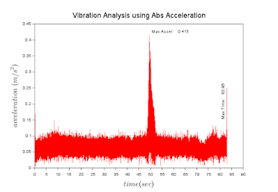
Here is the Scilab script for visualization of the example downloaded data from the Phyphox app.  The app’s acceleration data is organized into five columns: time, accel x-axis, accel y-axis, accel z-axis, and accel abs.  An example plot of the time and accel abs (absolute acceleration) and its script are presented.

Scilab Script

// Plotting data from accelerometer using Phyphox & Scilab
// by: Gani Comia, Aug. 2024
clear;clc;

// extracting data
clear importdata;

function [data]=importdata(filename)
    data = csvRead(filename, ",", ".", "double")
endfunction

[A] = importdata("accelerometerData.csv");

// assigning variable name
time = A(:,1);
accel_x = A(:,2);
accel_y = A(:,3);
accel_z = A(:,4);
accel_abs = A(:,5);

maxTime = max(time);
maxAccel = max(accel_abs);
disp(maxTime,maxAccel)

// plotting acceleration data
clf;
f=gcf();
f.figure_size=[700,600];
plot(time,accel_abs,"red")
title("Vibration Analysis using Abs Acceleration","fontsize",4)
xlabel("$time (sec)$","fontsize",4)
ylabel("$acceleration\;(m/s^2)$","fontsize",4)

// displaying information
format("v",6)
xstring(50,maxAccel,["Max Accel:", string(maxAccel)])
xstring(maxTime,0.15,["Max Time:", string(maxTime)],-90)

Executing the script will give you the plot for visualization of the acceleration data.

Fig. 1. Vibration Analysis using Absolute Acceleration.

The Scilab simulation tool facilitates visualization of numerical data, as in this case the acceleration of the vibrating object. Further numerical analysis to determine the velocity, displacement, and frequency of vibration can be done as well using the tool.

Feel free to comment for inquiry, clarification, or suggestion for improvement. Drop your email to request the softcopy of the file.


Saturday, 23 November 2024

Spring Simulation with Cantilever Beam Deflection Formulae using Scilab

Topic: Mechanical Spring Simulation;

Subject: Machine Design & Strength of Materials;

Tool: Scilab;

by: Gani Comia, Nov. 2024;

Beam deflection formulae of the cantilever with the concentrated load \(P\) at the free end can also be a useful tool in analyzing a mechanical spring that resembles a cantilever.

In this example, a clip spring that resembles a cantilever was simulated to determine how much load is needed to reach the maximum deflection of \(\text{0.5 mm}\). The material being considered for the application was stainless steel, \(\text{SUS304}\). Simulation also shows the deflection profile at each section of the length.

Below is a free-body diagram (FBD) of the clip spring design.

Fig.1. Clip Spring Design FBD

The following formulas for maximum deflection and deflection at any section in terms of \(x\) of the cantilever beam were applied in the analysis.

Maximum deflection.

$$\delta_{max}\;=\;\frac{P\,l^3}{3\,E\,I} \tag{1}$$

Deflection at any section in terms of \(x\).

$$y(x)\;=\;\frac{P\,x^2}{6\,E\,I}\;\left(3\,l\,-\,x\right) \tag{2}$$

Simulation using Scilab Script.

// Clip Spring Simulation
// using Cantilver Beam Deflection Formulas
// by: Gani Comia, Jul. 2017
clear;clc;

// Input:  Clip Spring Parameter
E = 806e+3;             // MPa, modulus of elasticity, SUS304
l = 12;                 // mm, length
b = 10;                 // mm, width
t = 0.3;                // mm, thickness
I = (b.*t.^3)./ 12;     // mm^4, moment of inertia

// Calculation:  Force-deflection characteristics
delta = 0.0:0.01:0.5;               // mm, deflection (allowable)
P = ((3 .*E.*I.*delta)./ l.^3);     // N, load
maxP = -max(P)                      // N, max force, downward

// Calculation: Deflection at the given length
x = 0:0.1:12;                              // mm, section length
y = (maxP.*x.^2 .* ((3*l)-x)) ./ (6*E*I);  // mm, deflection

// Visualization:
clf;
f=gcf();
f.figure_size=[600,650];

// Plot of delta vs. load
subplot(2,1,1);
plot(delta,P,"-b","linewidth",2.2);
title("Force - Deflection (SUS Clip Spring)");
xlabel("Deflection (mm)");
ylabel("Force (N)");
xstring(0.3,13.5,["Fmax:",string(max(P)),"N"]);
xgrid(12,0);

// Plot of length vs. deflection
subplot(2,1,2)
plot(x,y,"-r","linewidth",2.2);
title("Deflection - Length (SUS Clip Spring)");
xlabel("Length Segment (mm)");
ylabel("Deflection (mm)");
xgrid(12,0);

Shown is the simulation plot.


Fig. 2. Mechanical Spring as Cantilever Beam Simulation.

The Scilab simulation tool facilitates visualization of the reaction of a machine element to a given load. A machine designer might evaluate a range of attributes in their decision-making process.

Feel free to comment for inquiry, clarification, or suggestion for improvement. Drop your email to request the softcopy of the file.


Thursday, 21 November 2024

Plotting Position, Velocity & Acceleration as a function of Time

Topic: Position, Velocity & Acceleration Plot as a Function of Time

Subject: Numerical Methods & Kinematics

Tool: Scilab

by: Gani Comia, Nov. 2024

In the subject of kinematics, the position, velocity, and acceleration as a function of time can be plotted using the forward difference of the numerical method of differentiation. For a given position as a function of time, t, as represented by s = f(t), velocity and acceleration can be solved as s' = f'(t) and s'' = f''(t), respectively.

The Scilab "diff()" function facilitates the numerical differentiation of a given function.

Below is an example of a Scilab script to make a plot of position, velocity, and acceleration as a function of time.

Scilab Script.

// Copyright (C) 2024 - Gani Comia
// Date of creation: 21 Nov. 2024
// Position, Velocity & Acceleration as a function of time
clear;clc;
// Given: Position as a function of time, t.
// s(t)=3t^4 - 35t^3 + 120t^2 - 10

function s=f(t)
    s = 3*t.^4 - 35*t.^3 + 120*t.^2 - 10
endfunction

dt = 0.01                   // time step, dt
t = 0:dt:5                  // time range, t
s = f(t)                    // position, s
v = diff(s)/dt              // velocity, ds/dt (s')
a = diff(s,2)/dt.^2         // acceleration, d2s/dt2 (s'')

clf;
f = gcf()
f.figure_size = [600,700]

// position vs time plot
subplot(3,1,1)
plot(t,s,"-r","linewidth",2.5)
title_1=["Position ,", "$s=3\;t^4-35\;t^3+120\;t^2-10$"]
title(title_1, "fontsize",3)
ylabel("position, s")
xgrid()

// velocity vs time plot
subplot(3,1,2)
plot(t(1:$-1),v,"-b","linewidth",2.5)
title_2=["Velocity ,", "${ds}\;/\;{dt}$"]
title(title_2,"fontsize",3)
ylabel("velocity, v")
xgrid()

// acceleration vs time plot
subplot(3,1,3)
plot(t(1:$-2),a,"-g","linewidth",2.5)
title_3=["Acceleration ,", "${d^2s}\;/\;{dt^2}$"]
title(title_3,"fontsize",3)
ylabel("acceleration, a")
xlabel("time, t","fontsize",2)
xgrid()

Below is the graph as a result of running the Scilab script.

Fig. 1. Graph of Position, Velocity & Acceleration as a function of Time. 

Feel free to comment for inquiry, clarification, or suggestion for improvement. Drop your email to request the soft copy of the file.


Sunday, 17 November 2024

Pumps Total Dynamic Head (TDH) and Pressure using EMT

Topic: Visual Plot of Pump's Pressure Head and Volumetric Flow;

Subject: Fluid Mechanics;

Tool: Euler Math Toolbox;

by: Gani Comia, Nov. 2024;

In one scenario, a 100 GPM volumetric flow of water is being required in a building's fire protection system. Your facility manager is asking if it can be achieved from existing < 70 GPM and if the pressure setting can be adjusted from the current 100 psi to something like 160 psi. As a technical resource person in mechanical, you need to provide an explanation with the supporting calculation and visual simulation in layman's terms.

EMT Script

Pumps Total Dynamic Head & Pressure

The pump's horsepower (HP) is calculated from a given volumetric flow rate (Q) of fluid and the total dynamic head (H):

To determine the total dynamic head (TDH), H:

Solution:

>HP = 10+2.5;         // hp, e.g. fire pump + jockey pump
>Q  = 50:120;         // gpm, volumentric flow from 50 to 100
>e  = 0.80;           // %, efficiency (assumed)
>H  = (1714*HP*e/Q);  // ft, total dynamic head

Pressure head calculation:

where:

>gamma = 62.4;        // lb/ft^3, weight density of H2O
>h = H;               // ft, pressure head
>P = (gamma*h)/144;   // psi (from lb/ft^2), pump pressure

Data Visualization:

>aspect(1);
>plot2d(P,Q,title="Fire & Booster Pump Characteristic", ...
 xl="Pump Pressure [psi]",yl="Pump Vol. Flow [gpm]");

Shown in fig. 1. is plot generated by EMT script.

Fig. 1. Visual representation of the pump's characteristics.

Feel free to comment for inquiry, clarification, or suggestion for improvement. Drop your email to request the softcopy of the file.


Saturday, 16 November 2024

Pipe Leak Rate due to Pressure Drop using EMT

Topic: Pipe Leak Rate due to Pressure Drop;

Subject: Fluid Mechanics or Hydraulics;

Tool: Euler Math Toolbox (EMT);

by: Gani Comia, Nov. 2024;

This handy calculation toolbox was created to estimate the water leak rate due to pressure drop in a firefighting system of a building. The situation here was that the fire pump automatically shuts off after reaching the 100 psi high pressure setting. It was observed that the pressure was dropping down with all the gate valves closed. The pressure reached 20 psi in just 18 minutes. 

Below is an estimation of the water leak rate using EMT.

EMT Script.

Pipe Leak Rate due to Pressure Drop

The leak rate calculation for incompressible fluid due to pressure drop is:


Given:

>p1 = 100*6.9;                // kPa (100 psi), initial pressure
>p2 = 20*6.9;                 // kPa ( 20 psi), final pressure
>t  = 18;                     // min, time duration of pressure drop

Pipe network data.
Pipe size : Dia 38mm GI Pipe S40
Pipe length : 342 m

>pipeId = (38-2*1.5)/1000;       // m, inside dia, GI pipe S40 38mm
>areaId = (1/4)*%pi*(pipeId)^2;  // m^2, area, GI pipe S40 38mm
>pipeLg = 342;                   // m, total pipe length
>V  = areaId*pipeLg;             // m3,  volume of system under test

Leak rate calculation.

>function Q(p1,p2,V,t) := ((p1-p2)*V)/t

Leak rate, [L/min].
Note: 1 kPa m^3 ~ 1 Liter

>leakRate = Q(p1,p2,V,t);
>"Leak rate: " + leakRate + " L/min for 1 kPa pressure drop."
Leak rate: 10.0906385237 L/min for 1 kPa pressure drop.

Feel free to comment for inquiry, clarification, or suggestion for improvement. Drop your email to request the softcopy of the file.


C++ and Python for Numerical Solution to Spring-Mass-Damper Model

Topic: SDOF Spring-Mass-Damper System Subject: Numerical Methods & Mechanical Vibration Tools: C++, CodeBlocks, GitHub Copilot, LabP...